
Distinguishing errors and uncertainties in design using chaotic simulation results

Advances in computational fluids have brought state-of-the-art computational science and engineering techniques for chaotic unsteady systems within an arm's reach of the industrial design process in aeronautics; in order to more completely integrate these into the simulation pipeline for design, we will want to incorporate them in a way that minimizes the error in these simulations per cost.
Simulations of Chaotic Systems
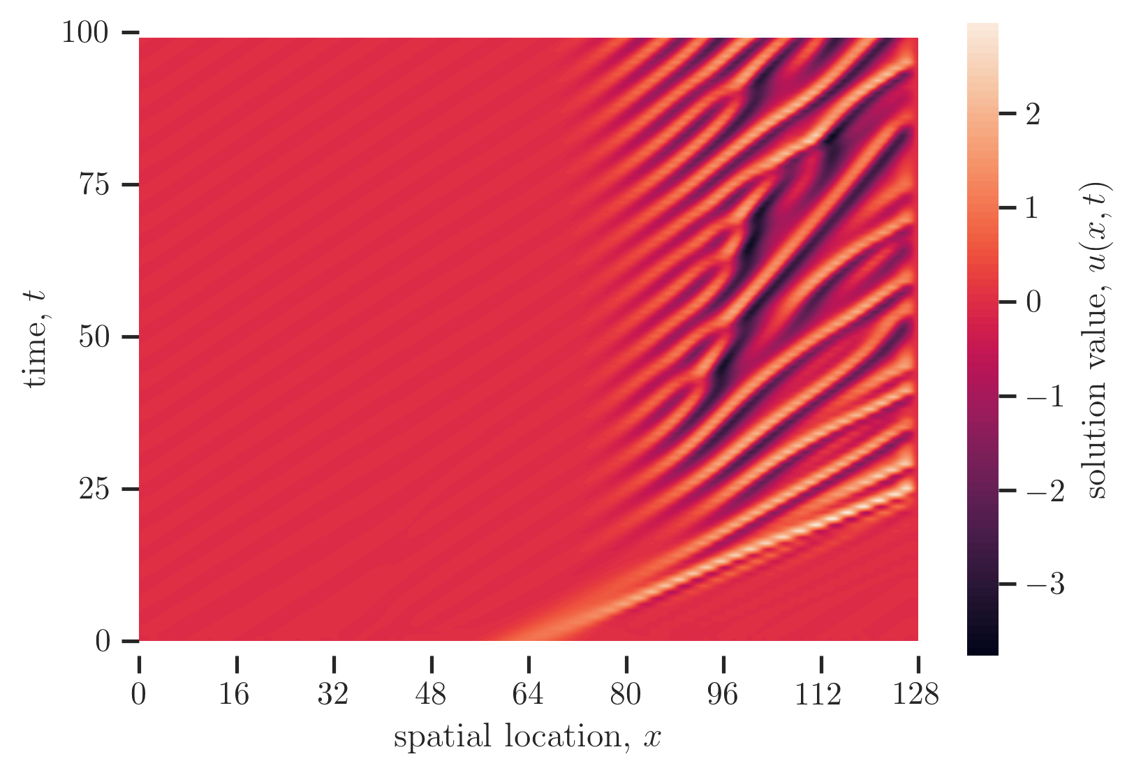
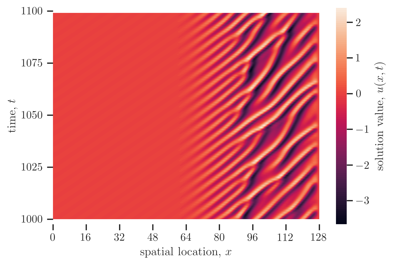
Consider a simulation of a chaotic PDE system, for an example (a relatively cheap one at that) the Kuramoto-Sivashinsky equation (KSE), which describes flame front propogation. A plot of the solution $u$ of the KSE is shown below, from time $t= 0$ to time $t= 100$ and from time $t= 1000$ to $t= 1100$:
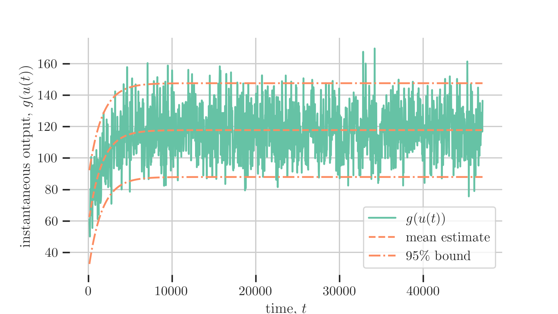
We might run a simulation of the Kuramoto-Sivashinsky equation in order to make estimates of the mean energy by averaging the instantaneous energy
$$
g(u(t))= \int_0^L u^2(\mathbf{x}, t) \mathrm{~d} \mathbf{x}
$$
the resulting estimate of the instantaneous energy is below, with a fit that captures the long-term statistical structure (mean and variance) as well as the transient behavior that decays away from the starting condition.
It is important to note that the physical system itself involves natural, deterministic variation. This variation, under natural assumptions about the ergodicity of the system, should result in states sampled from a stationary distribution with a well-defined mean and variance.
Corrolary to this assumption, finite-time averages of the true state, as
$$
J_T= \frac{1}{T_s} \int_{t_0}^{t_0 + T_s} g(u(\mathbf{x}, t)) \mathrm{~d} t
$$
should be drawn from a normal random variable with a standard deviation that scales with $T_s^{-1/2}$ under the Central Limit Theorem (CLT). The effect of this is that some expected error should be present in any estimate $J_T$ of the true system.
When a system like this is simulated by a discrete method, an additional error is incurred by the representation of the true solution by some discrete representation. In expectation, this error typically manifests in some offset or modification of the distribution of the mean value of the system. The approximation choices can be represented by a set of discretization scales $h$ and orders $p$, and the errors in an discrete approximation are expected to be determined by $h$, $p$, and the discretization, as well as by fundamental properties of the discretization and physical system. One possible form of this error is an offset
$$
e_{hp} \approx C h^q .
$$
where the grid length is given by $h$ and the order of convergence of the errors ( a constant) by $q$. In general $h$ will get larger as $T_s$ increases (holding computational costs constant) or smaller as the computational work per simulation instance increases (holding $T_s$ constant).
Categorization of uncertainties and errors
Uncertainties
In statistics and machine learning, a typical way of dividing uncertainties is into epistemic and aleatoric uncertainty. Suppose a pair of (possibly loaded) 6-sided dice is being rolled. The act of rolling the dice results in some outcome that is fundamentally stochastic and unpredictable. The actual likelihood of any given outcome of the diceroll (e.g. $(1, 1), (1, 2), \ldots, (6, 6)$) is a well-defined quantity, and with every new diceroll, of which we can make improved estimates. Even after an infinite number of rolls– and thus with these probabilities estimated perfectly– because of the underlying stochasicity of the next diceroll it can not be predicted. Thus, uncertainty about the likelihood of outcomes is reducible by the incorporation of new data, and we call this epistemic uncertainty. On the other hand, the uncertainty about the next outcome is irreducable, and referred to as aleatoric uncertainty.
Errors
Meanwhile, in discretized systems, there are numerous types of errors which themselves represent a form of uncertainty about the true answers. Truncation error occurs due to finite representation of functions, which nominally can be represented perfectly as "truncations" of e.g. infinite series of polynomials (subject to a collection of appropriate assumptions). Truncation errors propogate and accumulate over some time period to result in so-called "global discretization error", which typically for chaotic systems result in the form written above.
Moreover, if a system is ergodic, meaning it is unsteady but its solutions have a well defined mean value, then there will be some error in finite-length estimates of the mean, typically described by the Central Limit Theorem (CLT). Combining these errors leads to a total "simulation error" that should manifest asymptotically as a normally-distributed error with a finite, non-zero mean and variance, which get smaller as the grid scale $h$ shrinks or as the sampling time $T_s$ gets larger, respectively.
Classification of uncertainties in chaotic systems
The question at the heart of this blog post, then, is: if I simulate a chaotic system as part of a design pipeline, what errors are aleatoric and which are epistemic? Or, what is reducible, and how should I concentrate the effort to reduce the uncertainty in a design quantity of interset? The answer is not so clear. Many treatments of discrete results in statistics treat uncertainties due to discretization errors as irreducible, but the allocation of more computational work per instance would reduce the global discretization error (and therefore reduce uncertainty). Likewise, if we're talking about averages, increasing sampling time $T_s$ also can close in the uncertainty from natural variation. Point being: in computational practice these factors will be competing for resources, and it's important to take a wholistic view of how to reduce the uncertainties that are most important in order to maximize benefit of computation in the design cycle.