Output error behavior for discretizations of ergodic, chaotic systems of ordinary differential equations

This post is a summary of my Sept. 2022 publication of the same name in Physics of Fluids, which was a featured article in PoF around that time; this paper is also, effectively, a slightly modified version of the first chapter of my Ph.D. thesis.

Intro

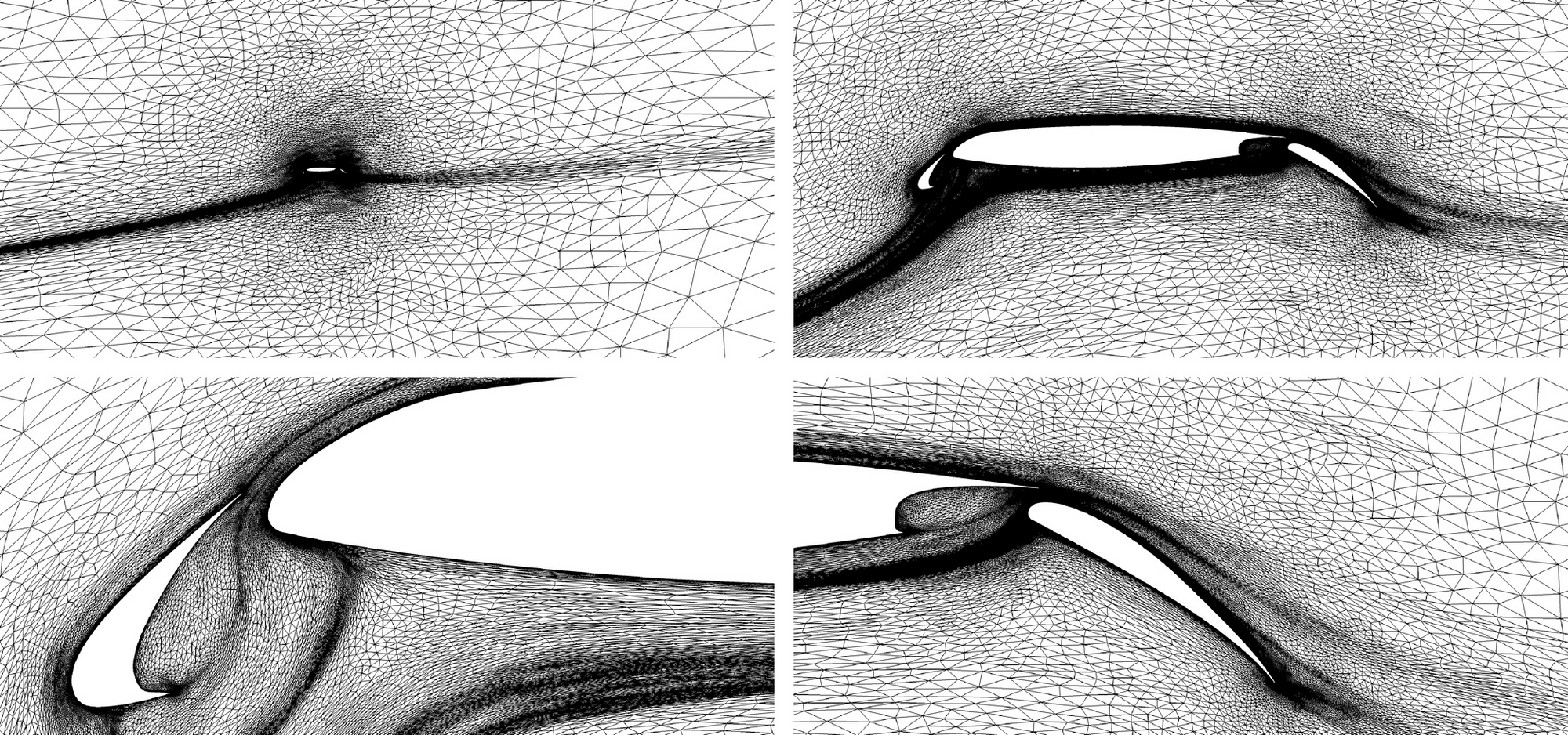
One problem in computational methods for engineering is that we're interested in simulating complex^[1] systems, not just simple ones. Systems can be complex in a lot of different ways. Consider the flow around an airfoil; in many cases, the mean flow can be very well approximated by steady-state equation. Even when this is the case, the regions around the airfoil that are more or less important are not easy to predict. In order to generate predictions of the flow around the airfoil without knowing it in the first place, one possibility is adaptive meshing, shown in the image above, taken from Michal, et. al (2021). Coupled with so-called high-order finite element methods, adaptive meshing allows for significant improvement in the relationship between error and computational costs for systems that can be described in a steady form.

Another layer of complexity arrives when systems can no longer be described accurately by a steady form of equations, such as when flow "separates" or "detaches" from the sutface of the airfoil. In this case, the simulation must be unsteady, fully resolving the temporal variations in the system. This can lead-- and often does lead-- to the onset of turbulent and therefore chaotic dynamics. Chaotic systems are characterized by ([https://doi.org/10.1201/9780429492563](Strogatz Nonlinear dynamics and chaos (2001))):

1. purely deterministic physics
2. aperiodic, oscillatory solutions
3. sensitive dependence on initial conditions

In simpler terms: chaotic systems present a challenge for simulation, since not only are they complex in the sense that the struture of the solutions are unknown, but chaotic systems don't have predictable or unique solutions.

This leaves us with a key question: what does it mean to have a good discretization of a chaotic system, and how do we achieve it? The goal of this work is to begin to answer that question.

Error modeling

While the solutions of chaotic problems are effectively random, most problems of interest have unique long-term averages of quantities of interest^[1], and these are typically the target quantity of a simulation. We can denote these true, long-term averaged quantities using $J_\infty$, and express the concept mathematically as:
$$
J_\infty = \lim_{T \to \infty} \frac{1}{T} \int_{t_0}^{t_0 + T} g(\mathbf{u}(t)) ~\mathrm{d} t .
$$

In practical terms, we can only make a simulation of the system that runs for a finite time and using a discrete approximation of the physical system. We can refer to such a result by the term $J_{T,hp}$ with the subscript $T$ referring to sampling on a finite time $T_s$ and the subscript $hp$ referring to the discretization size $h$ and the approximating order $p$.
We express this mathematically by:
$$
J_{T,hp} = \frac{1}{T_s} \int_{t_0}^{t_0 + T_s} g_{hp}(\mathbf{u}_{hp} (t)) ~\mathrm{d} t ,
$$
where $\mathbf{u}_{hp}$ and $g_{hp}$ represent discrete approximations of the state of the system and the output functional of interest.

The novel contribution of this work comes from introducing a third quantity: the true, finite time average of the system, or $J_T$:
$$
J_T = \frac{1}{T_s} \int_{t_0}^{t_0 + T_s} g(\mathbf{u}(t)) ~\mathrm{d} t .
$$
This quantity doesn't have a unique value, but for many systems of interest^[2], the average difference $e_T= J_T - J_\infty$ should be a random quantity governed by the central limit theorem from 101-level statistics.

Meanwhile, the difference between $e_{hp}= J_{T,hp} - J_T$ should be governed by classical discretization theory^[3]! Now, a simple set of relations can be used to describe the error in approximating $J_\infty$ by $J_{T,hp}$:
$$
\begin{aligned}
e_{T,hp} &= \left| J_{T,hp} - J_\infty \right| \\
&= \left| (J_{T,hp} - J_T) + (J_T - J_\infty) \right| \\
&= \left| e_T + e_{hp} \right| \\
|e_{T,hp}| &\leq |e_T| + |e_{hp}|
\end{aligned}
$$

Last but not least, since any given solution is effectively random, so is $J_{T,hp}$. What we are interested in is the expected value of the error quantities, what they would be over a sampling of all of the trajectories of the chaotic system. Denoting by $\mathbb{E}[\cdot]$ an appropriate expectation, we arrive at a model for the expected error in a simulation:
$$
\begin{aligned}
\mathbb{E}[|e_{T,hp}|] &\approx \mathbb{E}[|e_{hp}|] + \mathbb{E}[|e_T|] \\
& \approx e_\mathrm{model} \equiv C_q \Delta t^q + A_0 T_s^{-1/2}
\end{aligned}
$$
where $C_q$, $q \approx p$, $A_0$, and $r \approx 1/2$ are constant parameters for a given system & discretization. Thus: we can characterize the expected errors by ths equation if we can describe these variables!

Experiments

Next, we do a bunch of experiments to show that this model applies to a simple chaotic problem. For a problem we use the Lorenz system, and attempt to approximate the long-term average of its vertical location. We run a huge number of very long simulations to establish a very-accurate estimate $J_\mathrm{ref} \approx J_\infty$. Then, we run a lot of simulations at various values of $\Delta t$ with $T_s= N_s \Delta t$ set by a fixed budget of timesteps $N_s$; the result is plots of the error model as a function of $\Delta t$, like in Figure 5 below, sets $N_s$ such that runtime across different discretization methods is similar.

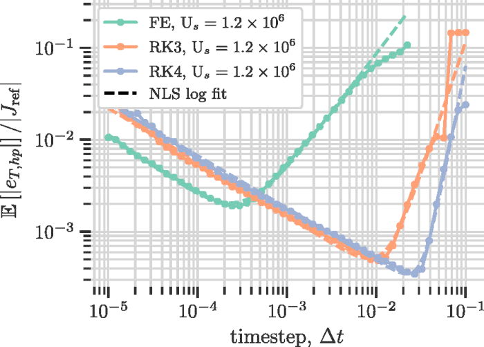
The important conclusion of this plot is that if you want to minimize the error you'd expect from a simulation there is a particular choice of $\Delta t$ (and therefore $T_s$ that you would use to do it. And the modeling framework we've described here can find it... if you know the governing constant parameters. Unfortunately, they're not typically known and there's little point in running exhaustive studies to find them.

Model implications

Nonetheless, this model gives a framework for understanding the accuracy of estimates of $J_\infty$ that might possible at a fixed cost. Leaving a number of details to the text, we can show that the best possible scaling of the error under the model is given by:
$$
e_\mathrm{model} \sim N_s^{-\frac{q}{2q+1}} \leq N_s^{-1/2}
$$

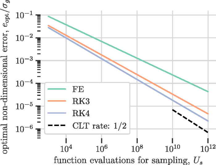
This implies that, in the limit of perfect discretization, the best estimate you can achieve of $J_\infty$ behaves as the central limit theorem predicts. Moreover, the effect of discretization errors are to dilute this rate. We can see this in Fig. 12 of the paper, shown below, which shows the long-run error convergence of different methods, which converge towards the CLT-predicted rate.

Model enhancements: spin-up transients and Monte Carlo estimators

The last effort in the paper is to consider the behavior of a chaotic system where two additional features of interest to computational fluid dynamics researchers in particular: spin-up transients and ensemble Monte Carlo simulations for estimation of $J_\infty$.

In brief, the findings of this final section of the paper boil down to two observations. For one, the resolution of startup transients must be handled on each instance, so it doesn't parallelize, and when it's the dominant factor convergence behavior will be limited by the need to handle it. Second, when sampling is a dominant cost, the parallelization can reduce the error at a given amount of cost by a factor $\sqrt{M_\mathrm{ens}^{-1}}$, as in the canonical central limit theorem, assuming the instances can be made to be effectively random draws. As before, the error model can give optimal choices of discretization at fixed computational cost, now balancing $\Delta t$, $T_s$, and spin-up time $t_0$, but as observed previously the best-possible convergence rate is the CLT's rate of $1/2$.

Conclusions

Overall this paper contributes to the literature a comprehensive error and cost modeling approach for chaotic ODE systems and offers an outline of how one might attack characterization of the error for a chaotic PDE problem. It gives a somewhat pessimistic view of convergence rates possible for estimation of averaged quantities of interest, limited by the central limit theorem. Finally, it leaves a big question outstanding: what are we supposed to do knowing these error behaviors exist but remain unknown before we run a simulation? Is there a way to work in an optimal way with respect to these errors without a priori knowledge?